This notebook shows a general example of mass balance calculation, we currently support two algorithms:

1. Non-negative algorithm, it solves KKT (Karush-Kuhn-Tucker) conditions for the non-negative least squares problem

2. Matrix decomposition, following Li et al. (2020) and Ghiorso 1983. The compositional matrix will be broken down by singular value decomposition, the coefficients will then calculated.

# import python modules
import pandas as pd
import matplotlib.pyplot as plt
from massbalance.mb_tools import MassBalance

1. Define elements for calculation

We first need to define element list for mass balance calculation, special attention goes to FeO term, which we use FeO, not FeOt nor FeOtot, this is consistent with the input excel files. Feel free to change the order of the elements

cmpnts = ['SiO2','Al2O3', 'TiO2', 'MgO', 'FeO', 'MnO',  'CaO', 'Na2O', 'K2O', 'P2O5', 'Cr2O3']  # change your desired elements for mass balance calculation

if you also want to integrate standard deviation on elements, this can be done manually or by the following line

cmpnts_std =[x + '_std' for x in cmpnts]  # save columns for std
cmpnts_std

['SiO2_std',
 'Al2O3_std',
 'TiO2_std',
 'MgO_std',
 'FeO_std',
 'MnO_std',
 'CaO_std',
 'Na2O_std',
 'K2O_std',
 'P2O5_std',
 'Cr2O3_std']

2. Load data

The easist way is to copy paste data in the input excel file, please also check README file for details of data prepration

nat_comp = pd.ExcelFile("input_comp.xlsx")

We load the whole excel spreadsheet to a pandas ExcelFile, to access data in your spreadsheet, you can do so by looping through ExcelFile to a dictionary:

nat_dict = {}  # create dictionary to collect compositions of different phases
nat_phases = []  # create list to save all phases in the calculation. Note bulk will be the bulk compsition, run_index will be your sample number, or rock id . etc
for sheet_name in nat_comp.sheet_names:
    nat_phases.append(sheet_name)
    nat_dict[sheet_name] = nat_comp.parse(sheet_name)

nat_phases stores the sheet names, nat_dict stores the data of each sheet.

nat_phases

['gl', 'ol', 'sp', 'py', 'pureFe', 'pureNa', 'bulk', 'run_index']

Use the sheet name to access data, let’s what we have in the gl phase

nat_dict['gl'].head()

	Run_no	SiO2	Al2O3	P2O5	CaO	FeO	Na2O	MgO	TiO2	K2O	...	Al2O3_std	P2O5_std	CaO_std	FeO_std	Na2O_std	MgO_std	TiO2_std	K2O_std	MnO_std	Cr2O3_std
0	02As1	46.66	10.16	0.17	11.64	13.06	1.95	13.15	2.43	0.49	...	0.17	0.10	0.22	0.34	0.10	0.26	0.20	0.04	0.04	0.04
1	01As1	46.96	10.34	0.20	11.81	13.21	1.84	12.16	2.53	0.44	...	0.11	0.07	0.20	0.21	0.10	0.12	0.14	0.05	0.03	0.08
2	04As1	47.20	10.80	0.23	12.13	12.77	1.87	11.04	2.65	0.48	...	0.11	0.05	0.21	0.45	0.14	0.09	0.16	0.05	0.05	0.03
3	03As1	48.38	11.36	0.18	12.63	13.03	1.42	10.35	2.54	0.43	...	0.16	0.06	0.12	0.27	0.07	0.19	0.27	0.05	0.05	0.05
4	05As1	47.18	11.63	0.23	12.84	12.57	2.04	9.42	2.60	0.51	...	0.12	0.05	0.25	0.20	0.12	0.18	0.23	0.05	0.04	0.05

5 rows × 25 columns

we use run_index sheet to store all runs we wish to perform mass balance with, we can check by doing:

nat_dict['run_index']

	Run_no	T_C	fO2
0	02As1	1320	QFM
1	01As1	1302	QFM
2	04As1	1280	QFM
3	03As1	1260	QFM
4	05As1	1240	QFM
5	06As1	1200	QFM
6	15As1	1180	QFM
7	17As1	1170	QFM
8	14As1	1160	QFM

3. Mass balance calculation with MCMC progagting errors

MassBalance class does the core calculation. To start the calculation, we need to define the MassBalance class by passing all necessary infos for calculations: 1. input_comp – load the ExcelFile variable 2. comp_col – load element list 3. comp_std_col – load element std list (if avaiable), default is None 4. match_column – this is the column name that saves your expts run no., sample no., or rock id. in each spreadsheet 5. bulk_sheet – sheet name of which saves bulk composition(s) 6. index_sheet – sheet name stores entire infos about expts run numbers ± condition, sample numbers or rock id. 7. normalize – normalize your data to 100 during calculation, default is True

mb_cal = MassBalance(
    input_comp=nat_comp,
    comp_col=cmpnts,
    comp_std_col=cmpnts_std,
    match_column="Run_no",
    bulk_sheet="bulk",
    index_sheet="run_index",
    normalize=True,
)

mb_cal is a variable we create for mass balance calculation The calculation is done by calling the compute method in the MassBalance class as mb_cal.compute() Four parameters can be tuned during computing: 1. mc – define the number of MC calculations, the default is None, which will be a one time calculation 2. exportFiles – we can export the results to excel file output.xlsx and output_mean_median_std.xlsx. If mc is given, output_mean_median_std.xlsxstores statistical infos for mc results 3. batch_bulk: define if you have different bulk for each group of phases, this is useful for layers in layered intrusions or expts with variable starting compositions for different runs. If you only have one bulk composition, can turn it to False 4. method: use nnl for non-negative method, svd for matrix decomposition method

Below we give examples to perform 100 times MC calculation with non-negative method, export files, and we have pre-defined a batch bulk composition in the input file. More examples are given in the python scipt along with this code

res_dict = mb_cal.compute(mc=100, exportFiles=True, batch_bulk=True, method='nnl')

The result is saved in a python dictionary, with each key responses to the expts run no., sample no, or rock id you defined in the index sheet Let’s take a look the results of first experimental run 02As1

res_02As1 = res_dict['02As1']
res_02As1

	gl	ol	sp	py	pureFe	pureNa	r2	residues
0	0.980309	0.025299	0.0	0.0	0.0	0.000665	0.318216	0.101261
1	0.959695	0.031032	0.0	0.0	0.0	0.001112	1.174406	1.379230
2	0.979235	0.019375	0.0	0.0	0.0	0.002412	1.023295	1.047133
3	0.981838	0.011746	0.0	0.0	0.0	0.001503	0.629961	0.396851
4	0.968629	0.035022	0.0	0.0	0.0	0.000457	0.707438	0.500469
...	...	...	...	...	...	...	...	...
95	0.981687	0.022148	0.0	0.0	0.0	0.000000	1.030632	1.062203
96	0.980176	0.015765	0.0	0.0	0.0	0.000000	0.661183	0.437163
97	0.980972	0.025854	0.0	0.0	0.0	0.001035	0.950629	0.903696
98	0.974249	0.021821	0.0	0.0	0.0	0.000774	1.953085	3.814540
99	0.993793	0.003956	0.0	0.0	0.0	0.000000	0.733781	0.538435

100 rows × 8 columns

This is the MC results (100 times), to calculate statistical infos, you can simply call the built-in pandas functions as:

res_02As1.describe()

	gl	ol	sp	py	pureFe	pureNa	r2	residues
count	100.000000	100.000000	100.0	100.0	100.000000	100.000000	100.000000	100.000000
mean	0.981366	0.020590	0.0	0.0	0.000010	0.000551	0.876400	0.870697
std	0.009831	0.007873	0.0	0.0	0.000092	0.000666	0.321958	0.630622
min	0.957179	0.000337	0.0	0.0	0.000000	0.000000	0.275481	0.075890
25%	0.976014	0.015349	0.0	0.0	0.000000	0.000000	0.663642	0.440423
50%	0.981365	0.020979	0.0	0.0	0.000000	0.000344	0.812141	0.660398
75%	0.985775	0.025433	0.0	0.0	0.000000	0.000914	1.063028	1.130062
max	1.012758	0.042551	0.0	0.0	0.000910	0.002896	1.953085	3.814540

or only interested parameters

res_02As1.agg(['mean', 'median', 'std'])

	gl	ol	sp	py	pureFe	pureNa	r2	residues
mean	0.981366	0.020590	0.0	0.0	0.000010	0.000551	0.876400	0.870697
median	0.981365	0.020979	0.0	0.0	0.000000	0.000344	0.812141	0.660398
std	0.009831	0.007873	0.0	0.0	0.000092	0.000666	0.321958	0.630622

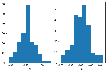
To plot the result, you can simply do:

fig, axes = plt.subplots(1,2, constrained_layout=True)
axes[0].hist(res_02As1['gl'], density=True)
axes[1].hist(res_02As1['ol'], density=True)
axes[0].set_xlabel('gl')
axes[1].set_xlabel('ol')
plt.show()

We pre-defined pure FeO and pure Na2O phases as the evaluation of Fe loss and Na loss, if you don’t want to check this, simply delete these sheets Below we give an example to calculate Fe loss (%) and Na loss (%) in the first experimental run 02As1

nat_bulk = nat_dict['bulk'].set_index('Run_no')
nat_bulk.loc['02As1', 'FeO']

12.42

nat_bulk.loc['02As1', 'Na2O']

1.96

res_02As1['Fe_loss'] = res_02As1['pureFe'] / nat_bulk.loc['02As1', 'FeO'] * 100 * 100
res_02As1['Fe_loss'].agg(['mean', 'median', 'std'])

mean      0.008275
median    0.000000
std       0.073758
Name: Fe_loss, dtype: float64

res_02As1['Na2O_loss'] = res_02As1['pureNa'] / nat_bulk.loc['02As1', 'Na2O'] * 100 * 100
res_02As1['Na2O_loss'].agg(['mean', 'median', 'std'])

mean      2.813345
median    1.756814
std       3.398196
Name: Na2O_loss, dtype: float64

Fin ~ happy coding!